---
title: "Binary Classification Model: Predicting Titanic Survivors with R"
subtitle: "Using Tidymodels"
execute:
warning: false
error: false
format:
html:
toc: true
toc-location: right
code-fold: show
code-tools: true
number-sections: true
code-block-bg: true
code-block-border-left: "#31BAE9"
---
## Introduction
This document provides a comprehensive, step-by-step guide to building a binary classification model using the `tidymodels` ecosystem in R. We will tackle the classic Titanic dataset, a rich collection of passenger data, to predict survival. This project will walk you through the entire machine learning pipeline, from initial data loading and exploratory data analysis (EDA) to sophisticated model training, hyperparameter tuning, and final model evaluation and deployment.
The primary goal is to demonstrate a robust and reproducible workflow for classification tasks. We will explore various algorithms, compare their performance, and select the best model for making predictions on unseen data.
## Installing and Loading Libraries
### Step 1: Install Necessary Libraries
First, we ensure that all the required R packages are installed. We use the `pak` package for efficient and reliable package management.
```{r}
#| label: install-packages
#| eval: false
# This chunk installs all necessary packages.
# It's set to not evaluate by default to avoid re-installing every time.
if (!requireNamespace("pak", quietly = TRUE)) {
  install.packages("pak")
}
# pak::pak handles dependencies gracefully.
pak::pak(c("tidymodels", "tidyverse", "titanic", "here", "naniar", "kableExtra", "ranger", "xgboost", "kknn", "kernlab", "doParallel", "discrim", "glmnet", "future.apply", "reactable", "skimr", "themis"))
```
### Step 2: Load Libraries
Next, we load the libraries that will be used throughout the analysis. Each library serves a specific purpose, from data manipulation (`tidyverse`) to modeling (`tidymodels`) and creating interactive tables (`reactable`).
```{r}
#| label: load-libraries
library(tidymodels)      # Core package for modeling
library(tidyverse)       # Data manipulation and visualization
library(titanic)         # Contains the Titanic dataset
library(here)            # For reproducible file paths
library(naniar)          # For visualizing missing data
library(kableExtra)      # For creating beautiful tables
library(discrim)         # For discriminant analysis models
library(glmnet)          # For regularized regression models
library(reactable)       # For interactive tables
library(future)          # For parallel processing
library(skimr)           # For summary statistics
library(themis)          # For dealing with imbalanced data
```
## Data Preparation
### Step 3: Read Data
We load the Titanic dataset, which is stored in a CSV file. The `here` package helps in locating the file relative to the project's root directory, making the code more portable.
```{r}
#| label: read-data
titanic_df <- read_csv(here("./data", "titanic_data.csv"))

# Glimpse the data to see its structure and variable types
glimpse(titanic_df)
```
### Step 4: Exploratory Data Analysis (EDA)
EDA is a crucial step to understand the data's underlying structure, identify missing values, and uncover relationships between variables.
```{r}
#| label: eda-summary
# Get a quick summary of the dataset
summary(titanic_df)
```
```{r}
# Use skimr for more detailed and user-friendly summary statistics
skim(titanic_df)
```
#### Automated EDA with `DataExplorer`
The `DataExplorer` package can generate a comprehensive HTML report, providing a deep dive into the data with a single command.
```{r}
#| label: dataexplorer-report
#| eval: false
# This command generates a detailed EDA report.
create_report(titanic_df, y = "Survived")
```
```{=html}
<iframe width="900" height="600" src="report.html" title="Auto EDA report"></iframe>
```
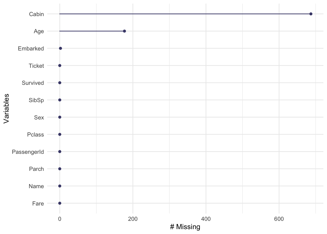
#### Visualizing Missing Data and Key Relationships
```{r}
# Visualize missing data to understand its extent
gg_miss_var(titanic_df)
```
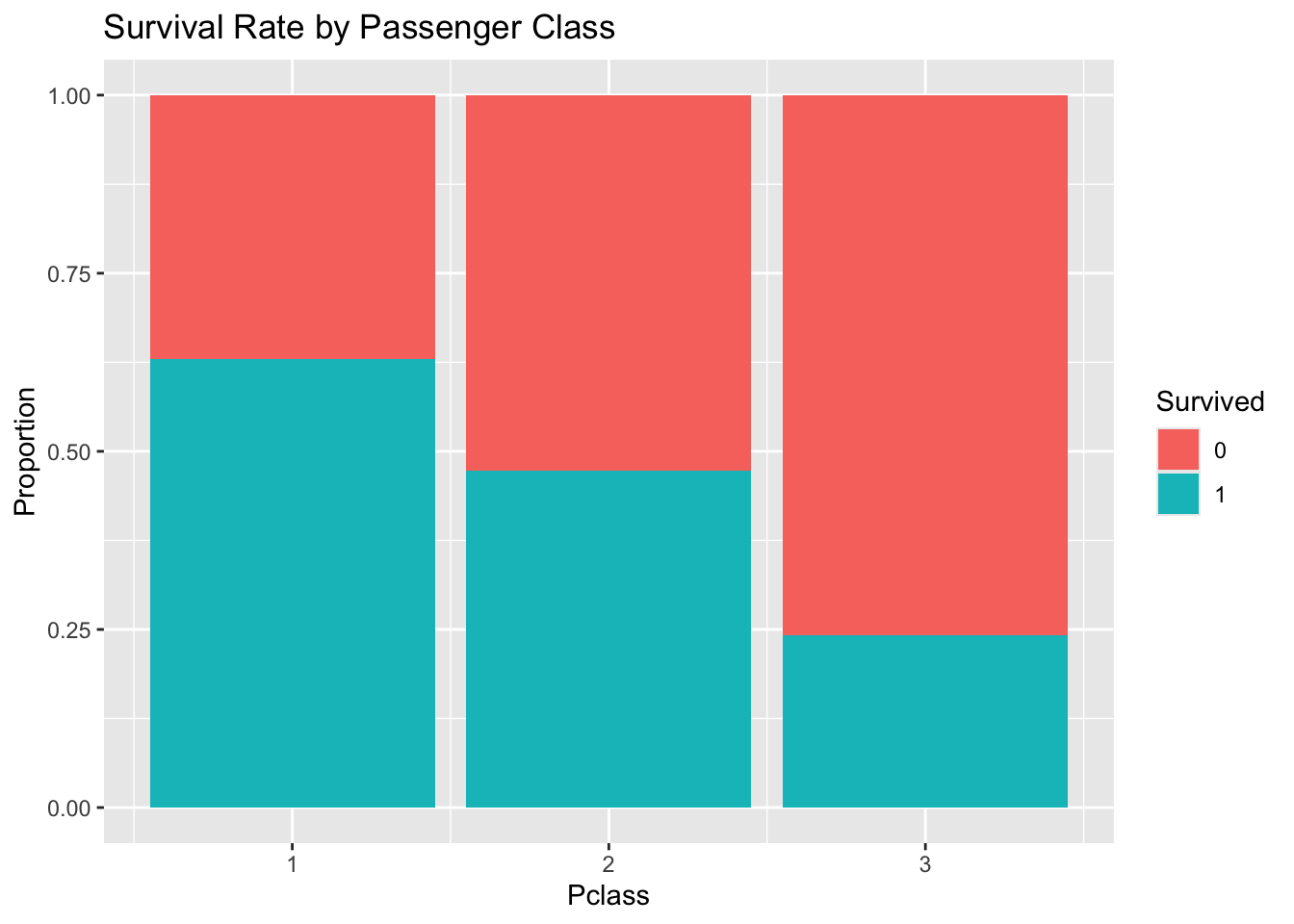
```{r}
#| label: eda-plots
# Explore survival rate by passenger class
titanic_df %>%
  mutate(Survived = as.factor(Survived)) %>%
  ggplot(aes(x = Pclass, fill = Survived)) +
  geom_bar(position = "fill") +
  labs(y = "Proportion", title = "Survival Rate by Passenger Class")
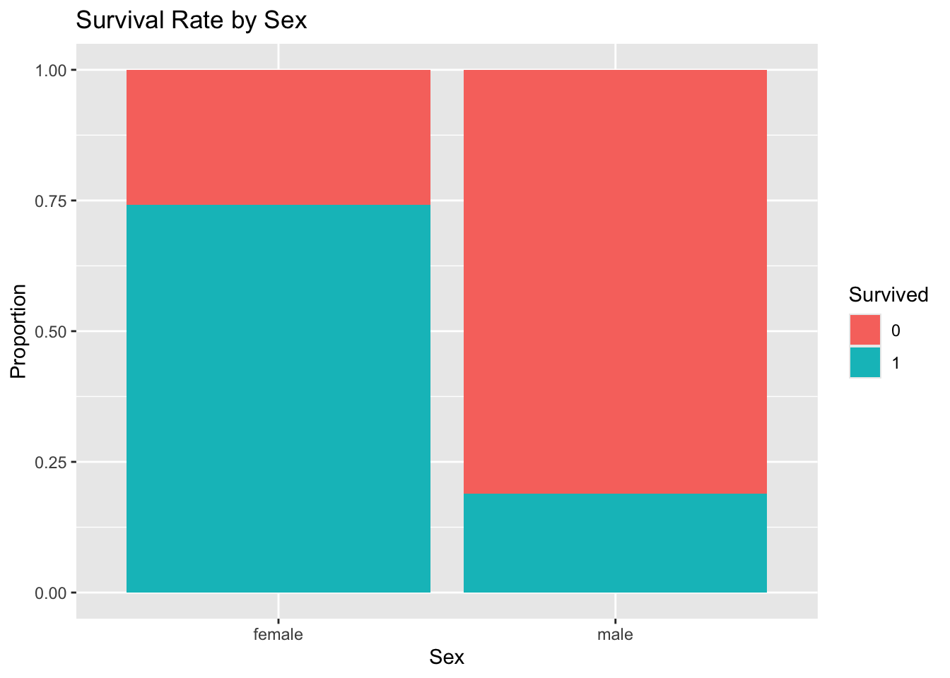
# Explore survival rate by sex
titanic_df %>%
  mutate(Survived = as.factor(Survived)) %>%
  ggplot(aes(x = Sex, fill = Survived)) +
  geom_bar(position = "fill") +
  labs(y = "Proportion", title = "Survival Rate by Sex")
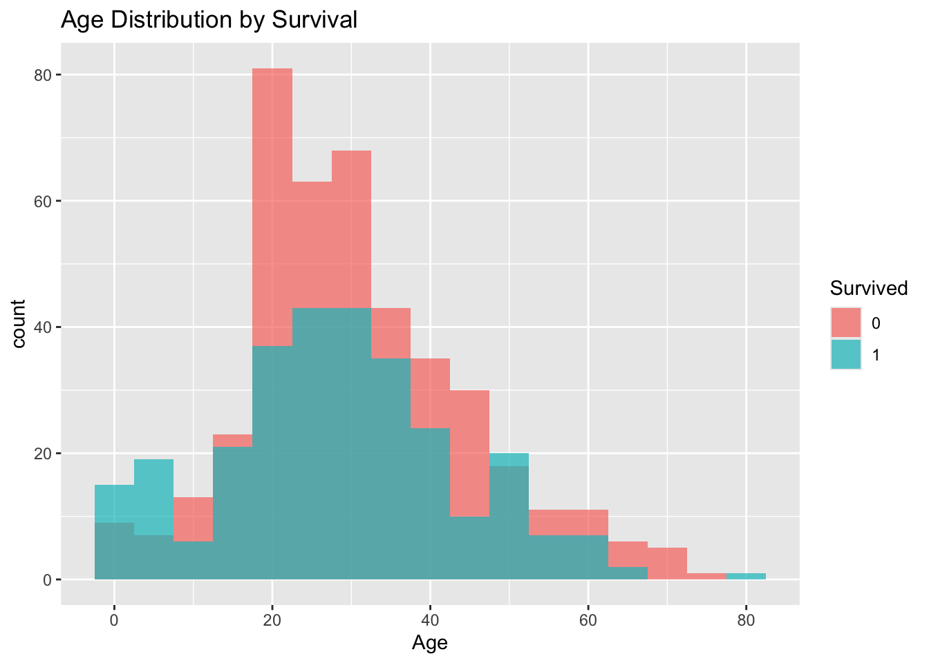
# Explore age distribution by survival
titanic_df %>%
  mutate(Survived = as.factor(Survived)) %>%
  ggplot(aes(x = Age, fill = Survived)) +
  geom_histogram(binwidth = 5, position = "identity", alpha = 0.7) +
  labs(title = "Age Distribution by Survival")
```
### Step 5: Data Cleaning and Feature Engineering
We perform some initial data cleaning, such as converting variables to the correct type. More complex preprocessing will be handled by the `recipe`.
```{r}
#| label: data-cleaning
titanic_clean <- titanic_df %>%
  mutate(
    Survived = as.factor(Survived),
    Pclass = as.factor(Pclass)
  ) %>%
  select(Survived, Pclass, Sex, Age, SibSp, Parch, Fare, Embarked, PassengerId, Name, Ticket)

titanic_clean$Pclass <- as.factor(titanic_clean$Pclass)
glimpse(titanic_clean)
```
#### Variable Groups
- **Target Variable**: `Survived`
- **Numerical Features**: `Age`, `SibSp`, `Parch`, `Fare`
- **Categorical Features**: `Pclass`, `Sex`, `Embarked`
- **Identifier Variables**: `PassengerId`, `Name`, `Ticket` (to be excluded from modeling)
### Step 6: Data Splitting
To properly evaluate our models, we split the data into three sets: a training set (for model building), a testing set (for tuning and initial evaluation), and a final hold-out set (for unbiased final validation).
```{r}
#| label: data-split
set.seed(123) # for reproducibility

# First, split into training/testing (90%) and hold-out (10%)
split_ho <- initial_split(titanic_clean, prop = 0.9, strata = Survived)
train_test_data <- training(split_ho)
holdout_data <- testing(split_ho)

# Next, split the 90% into training (7/9) and testing (2/9)
# This results in overall proportions of 70% train, 20% test
split_tt <- initial_split(train_test_data, prop = 7/9, strata = Survived)
train_data <- training(split_tt)
test_data <- testing(split_tt)

# Create cross-validation folds from the training data for robust evaluation
folds <- vfold_cv(train_data, v = 5, strata = Survived)

# Check the proportions of each dataset
cat("Training data:", nrow(train_data), "rows
")
cat("Testing data:", nrow(test_data), "rows
")
cat("Hold-out data:", nrow(holdout_data), "rows
")
```
```{r}
saveRDS(train_data, here("./data", "train_data.rds"))
saveRDS(test_data, here("./data", "test_data.rds"))
saveRDS(holdout_data, here("./data", "holdout_data.rds"))
```
## Modeling
### Step 7: Create a Preprocessing Recipe
A `recipe` is a powerful tool from `tidymodels` for defining a sequence of data preprocessing steps. This ensures that the same transformations are applied consistently to all data splits.
Our recipe will:
- Impute missing `Age` values using K-Nearest Neighbors.
- Impute missing `Embarked` values using the mode.
- Create dummy variables for all categorical predictors.
- Normalize all numeric predictors to have a mean of 0 and standard deviation of 1.
- Assign identifier roles to columns that should not be used as predictors.
```{r}
#| label: create-recipe
titanic_recipe <- recipe(Survived ~ ., data = train_data) %>%
  update_role(c(PassengerId, Name, Ticket), new_role = "sample ID") %>%
  step_impute_knn(Age, neighbors = 5) %>%
  step_impute_mode(Embarked) %>%
  step_dummy(all_nominal_predictors()) %>%
  step_normalize(all_numeric_predictors())

# Check the recipe to see the transformations
summary(prep(titanic_recipe))
```
```{r}
# Bake the recipe to see the transformed data
titanic_recipe %>% prep() %>% bake(new_data = test_data) %>% head() %>% glimpse()
```
### Step 8: Define Models
We will define a suite of classification models to compare their performance on this dataset.
#### Model Introductions
- **Logistic Regression**: A linear model that predicts the probability of a binary outcome. It's simple, interpretable, and a great baseline.
- **K-Nearest Neighbors (KNN)**: A non-parametric algorithm that classifies a data point based on the majority class of its 'k' nearest neighbors.
- **Support Vector Machines (SVM)**: A model that finds an optimal hyperplane to separate classes in the feature space. We'll use a radial basis function kernel.
- **Decision Trees**: A tree-like model of decisions. Simple to understand and visualize, but can be prone to overfitting.
- **Random Forest**: An ensemble of many decision trees. It improves upon single trees by averaging their results, reducing overfitting and increasing accuracy. We will tune its hyperparameters.
- **XGBoost**: An advanced and highly efficient implementation of gradient boosting. It's known for its high performance and is a popular choice in competitions. We will tune its hyperparameters.
- **Neural Networks**: A model inspired by the human brain, consisting of interconnected nodes (neurons) in layers. It can capture complex non-linear relationships.
- **Naive Bayes**: A probabilistic classifier based on Bayes' theorem with a 'naive' assumption of conditional independence between features. It is very fast and works well with high-dimensional data.
- **Regularized Logistic Regression**: An extension of logistic regression that includes a penalty term (L1/Lasso or L2/Ridge) to prevent overfitting by shrinking coefficient estimates. We will tune the penalty and mixture parameters.
#### Model Specifications
```{r}
#| label: model-specs
# Logistic Regression
log_reg_spec <- logistic_reg() %>%
  set_engine("glm") %>%
  set_mode("classification")

# K-Nearest Neighbors
knn_spec <- nearest_neighbor() %>%
  set_engine("kknn") %>%
  set_mode("classification")

# Support Vector Machine
svm_spec <- svm_rbf() %>%
  set_engine("kernlab") %>%
  set_mode("classification")

# Decision Tree
tree_spec <- decision_tree() %>%
  set_engine("rpart") %>%
  set_mode("classification")

# Random Forest (Tunable)
rf_spec <- rand_forest(
  mtry = tune(),
  trees = tune(),
  min_n = tune()
) %>%
  set_engine("ranger") %>%
  set_mode("classification")

# XGBoost (Tunable)
xgb_spec <- boost_tree(
  trees = tune(),
  tree_depth = tune(),
  min_n = tune(),
  learn_rate = tune(),
  loss_reduction = tune()
) %>%
  set_engine("xgboost") %>%
  set_mode("classification")

# Neural Network
nn_spec <- mlp(hidden_units = tune(), penalty = tune(), epochs = 100) %>%
    set_engine("nnet") %>%
    set_mode("classification")

# Naive Bayes
nb_spec <- naive_Bayes() %>%
  set_engine("naivebayes") %>%
  set_mode("classification")

# Regularized Logistic Regression (Tunable)
glmnet_spec <- logistic_reg(penalty = tune(), mixture = tune()) %>%
  set_engine("glmnet") %>%
  set_mode("classification")
```
#### Model Comparison Table
| Model | Key Strengths | Key Weaknesses | Tunable |
|---|---|---|---|
| Logistic Regression | Interpretable, fast, good baseline | Assumes linearity | No |
| K-Nearest Neighbors | Simple, non-parametric | Computationally intensive, needs scaling | No |
| SVM | Effective in high dimensions, robust | Can be slow, less interpretable | No |
| Decision Tree | Easy to interpret and visualize | Prone to overfitting | No |
| Random Forest | High accuracy, robust to overfitting | Less interpretable, can be slow | Yes |
| XGBoost | Top-tier performance, fast, flexible | Complex, many parameters to tune | Yes |
| Neural Network | Captures complex patterns, highly flexible | Requires large data, prone to overfitting | Yes |
| Naive Bayes | Very fast, works well on wide data | Strong feature independence assumption | No |
| Regularized Logistic Regression | Prevents overfitting, feature selection (Lasso) | Less interpretable than simple LR | Yes |
### Step 9: Create a WorkflowSet
A `workflow_set` is a powerful and convenient way to manage multiple workflows (recipe + model combinations) simultaneously, making it easy to train and compare them.
```{r}
#| label: create-workflowset
all_models <- list(
    log_reg = log_reg_spec,
    knn = knn_spec,
    svm = svm_spec,
    tree = tree_spec,
    rf = rf_spec,
    xgb = xgb_spec,
    nn = nn_spec,
    nb = nb_spec,
    glmnet = glmnet_spec
)

all_workflows <- workflow_set(
  preproc = list(recipe = titanic_recipe),
  models = all_models
)
```
### Step 10: Training and Hyperparameter Tuning
We use `workflow_map()` to efficiently fit the non-tunable models and tune the hyperparameters for the tunable ones using grid search. We'll leverage parallel processing to speed up this step.
```{r}
#| label: training
# Set up parallel processing to speed up computation
plan(multisession)

# Define the metrics we want to track
class_metrics <- metric_set(accuracy, roc_auc, sensitivity, precision)

# Tune the workflows using the cross-validation folds
set.seed(234)
tune_results <- workflow_map(
  all_workflows,
  "tune_grid",
  resamples = folds,
  grid = 15, # Use a grid of 15 candidate parameter sets for tuning
  metrics = class_metrics,
  control = control_grid(save_pred = TRUE) # Save predictions for later analysis
)
```
## Model Evaluation
### Step 11: Compare Model Performance
Let's visualize and compare the performance of all our trained models.
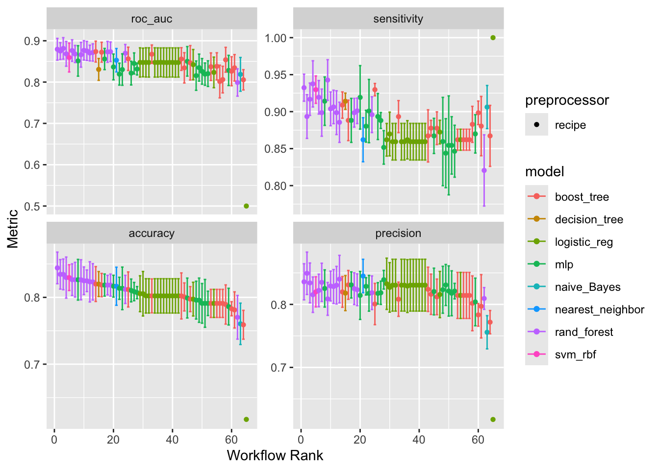
```{r}
#| label: show-performance
# Plot the results to visually compare model performance across metrics
autoplot(tune_results)
```
#### Understanding the Metrics
Before diving into the results, it's crucial to understand what each metric signifies. For binary classification, we often use a **confusion matrix** to evaluate a model's performance.
| | Predicted: Survived | Predicted: Perished |
|---|---|---|
| **Actual: Survived** | True Positive (TP) | False Negative (FN) |
| **Actual: Perished** | False Positive (FP) | True Negative (TN) |
- **AUC - ROC (Area Under the Receiver Operating Characteristic Curve)**: This is a key metric for classification. It measures the model's ability to distinguish between classes. An AUC of 1.0 is a perfect model, while 0.5 is no better than random chance.
- **Accuracy**: The proportion of correct predictions. It can be misleading if classes are imbalanced. `(TP + TN) / (TP + TN + FP + FN)`
- **Precision**: Of all passengers predicted to survive, how many actually did? `TP / (TP + FP)`
- **Recall (Sensitivity)**: Of all passengers who actually survived, how many did our model correctly identify? `TP / (TP + FN)`
```{r}
# Rank models by accuracy and display in an interactive table
rank_results(tune_results, rank_metric = "accuracy") %>%
  filter(.metric == "accuracy") %>%
  select(-n, -std_err, -preprocessor) %>%
  reactable(
    defaultPageSize = 10,
    striped = TRUE,
    highlight = TRUE,
    compact = TRUE,
    columns = list(
      wflow_id = colDef(name = "Workflow"),
      .metric = colDef(name = "Metric"),
      mean = colDef(name = "Mean", format = colFormat(digits = 4)),
      rank = colDef(name = "Rank")
    ),
    defaultSorted = list(rank = "asc")
  )
# Collect all metrics for further analysis
all_metrics <- collect_metrics(tune_results)
```
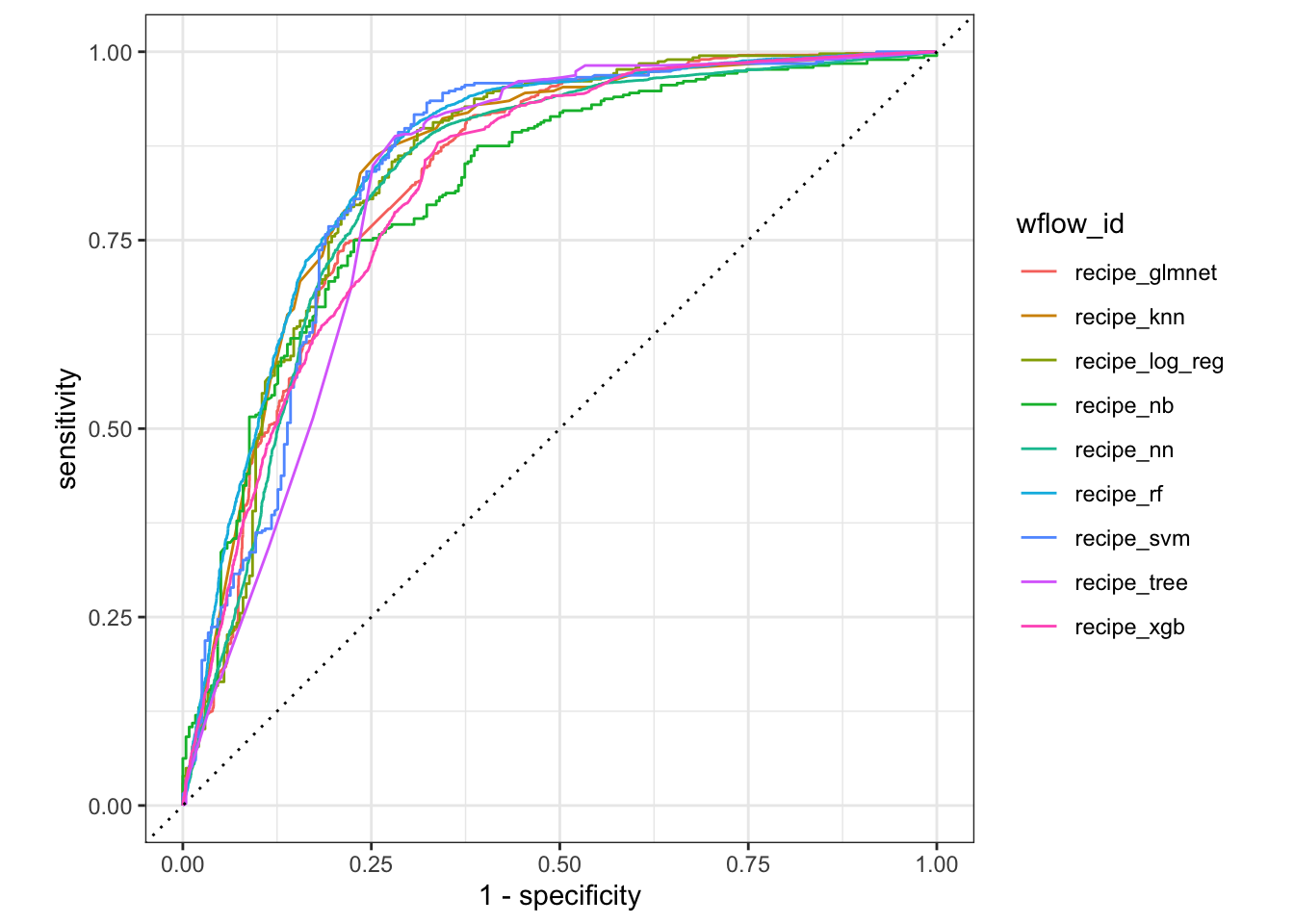
#### ROC Curves
We can plot the ROC curves for each model to visualize the trade-off between the true positive rate and the false positive rate.
```{r}
#| label: roc-curves
tune_results %>%
  collect_predictions() %>%
  group_by(wflow_id) %>%
  roc_curve(truth = Survived, .pred_0) %>%
  autoplot()
```
## Finalizing and Deploying the Model
### Step 12: Select and Save the Best Model
Based on our evaluation, XGBoost performed the best. We will now select this model, find its optimal hyperparameters, and fit it to the entire training and testing dataset.
```{r}
#| label: finalize-best-model
# Select the best workflow based on accuracy
best_wflow_id <- rank_results(tune_results, rank_metric = "accuracy") %>%
  dplyr::slice(1) %>%
  pull(wflow_id)

best_workflow <- extract_workflow(tune_results, id = best_wflow_id)

# Find the best hyperparameters for the top model
best_result <- extract_workflow_set_result(tune_results, id = best_wflow_id)
best_params <- select_best(best_result, metric = "accuracy")

best_params
# Finalize the workflow with the best parameters
final_workflow <- finalize_workflow(best_workflow, best_params)
final_workflow
# Fit the final model on the combined training and testing data
final_fit <- fit(final_workflow, data = train_test_data)

# Save the final fitted workflow including

# the fitted model
# the preprocessor (recipe)
# everything needed to predict

saveRDS(final_fit, file = here("./model/best_titanic_model.rds"))
```
### Step 13: Load the Saved Model
We can now load the saved model object for deployment or future predictions.
```{r}
#| label: load-model
loaded_model <- readRDS(here("./model/best_titanic_model.rds"))
#print(loaded_model)
summary(loaded_model)
```
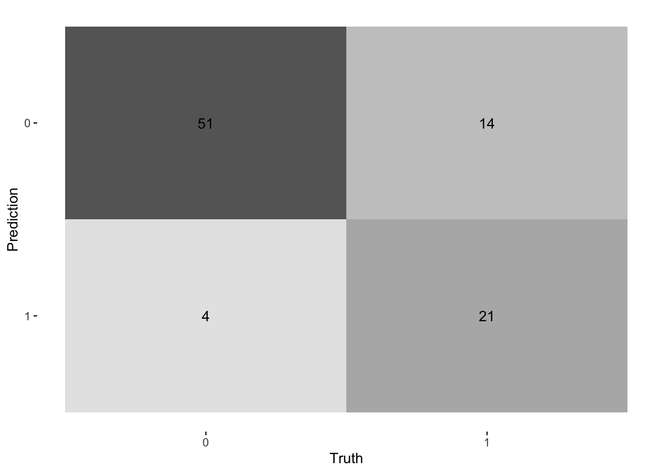
### Step 14: Make Predictions on Hold-out Data
Finally, we evaluate our best model on the hold-out data, which it has never seen before. This provides the most realistic estimate of its performance on new, unseen data.
```{r}
#| label: predict-holdout
# Make predictions on the hold-out set
holdout_predictions <- predict(loaded_model, new_data = holdout_data) %>%
  bind_cols(predict(loaded_model, new_data = holdout_data, type = "prob")) %>%
  bind_cols(holdout_data %>% select(Survived))

# Calculate performance metrics on the hold-out data
metrics <- metric_set(accuracy, precision, recall, f_meas, roc_auc)
final_performance <- metrics(holdout_predictions, truth = Survived, estimate = .pred_class, .pred_0)

# Display the final performance in a clean table
final_performance %>%
  kbl(caption = "Final Model Performance on Hold-out Data") %>%
  kable_styling(bootstrap_options = "striped", full_width = FALSE)
# Visualize the confusion matrix
conf_mat(holdout_predictions, truth = Survived, estimate = .pred_class) %>%
  autoplot(type = "heatmap")
```
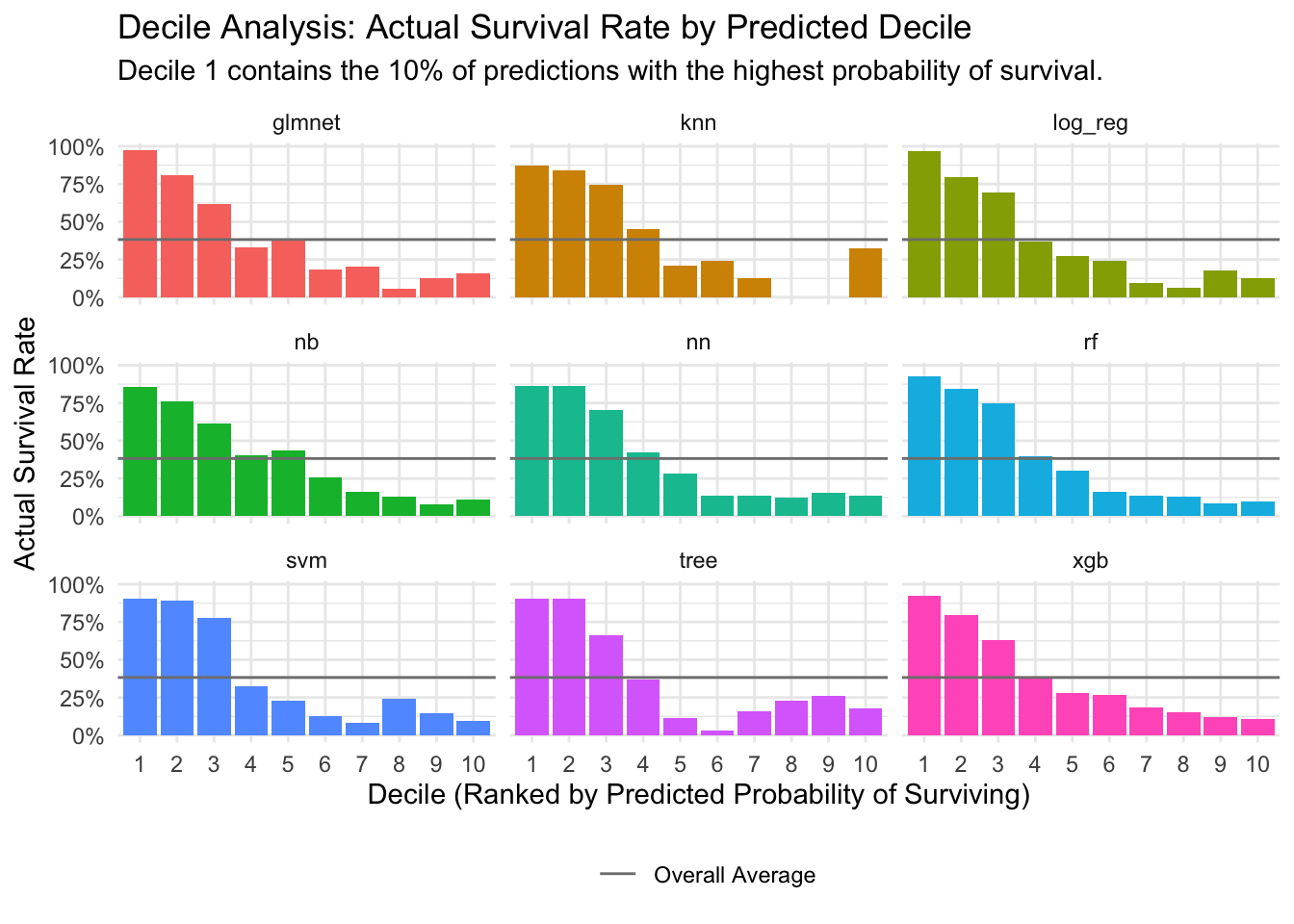
### Step 15: Decile Analysis
To better understand how well our models discriminate between classes, we perform a decile analysis. We sort predictions by the probability of survival, group them into 10 deciles, and then calculate the actual survival rate within each decile. This helps to visualize if the models are effectively identifying high-risk and low-risk groups.
```{r}
#| label: decile-analysis
# Get predictions from all models on the test set
all_predictions <- tune_results %>%
  collect_predictions()

# Calculate the overall average survival rate
overall_avg_survival <- mean(as.numeric(as.character(all_predictions$Survived)))

# Calculate deciles and survival rates for each model
decile_data <- all_predictions %>%
  mutate(Survived_numeric = as.numeric(as.character(Survived))) %>%
  group_by(wflow_id) %>%
  mutate(decile = ntile(desc(.pred_1), 10)) %>%
  group_by(wflow_id, decile) %>%
  summarise(
    avg_pred_prob = mean(.pred_1),
    actual_survival_rate = mean(Survived_numeric),
    n = n(),
    .groups = "drop"
  ) %>%
  mutate(wflow_id = str_remove(wflow_id, "recipe_"))

# Visualize the decile analysis
ggplot(decile_data, aes(x = as.factor(decile), y = actual_survival_rate)) +
  geom_col(aes(fill = wflow_id), show.legend = FALSE) +
  geom_hline(aes(yintercept = overall_avg_survival, linetype = "Overall Average"), color = "gray50") +
  scale_y_continuous(labels = scales::percent) +
  facet_wrap(~wflow_id, ncol = 3) +
  labs(
    title = "Decile Analysis: Actual Survival Rate by Predicted Decile",
    subtitle = "Decile 1 contains the 10% of predictions with the highest probability of survival.",
    x = "Decile (Ranked by Predicted Probability of Surviving)",
    y = "Actual Survival Rate",
    linetype = ""
  ) +
  theme_minimal() +
  theme(legend.position = "bottom")
```
## Conclusion
In this analysis, we successfully built and evaluated multiple machine learning models to predict Titanic survivors. The `tidymodels` framework provided a powerful and organized workflow for this task. Our final XGBoost model demonstrated strong performance on the hold-out data, indicating its effectiveness in this classification problem. This project serves as a template for tackling similar binary classification challenges in a structured and reproducible manner.